
Introduction
Traditional databases answer yes/no questions: does this record exist? Vector databases tackle a different challenge: which records are most similar to this? This shift is critical for modern data like images, text, and user behavior, which can’t be searched by exact matches. Instead of asking “find this,” we ask “find what is close to this.” Embedding models convert raw data into vectors, where geometric proximity equals semantic similarity. But scaling this to billions of vectors requires clever algorithms. Let’s break it down.
Level 1: The Core Similarity Problem
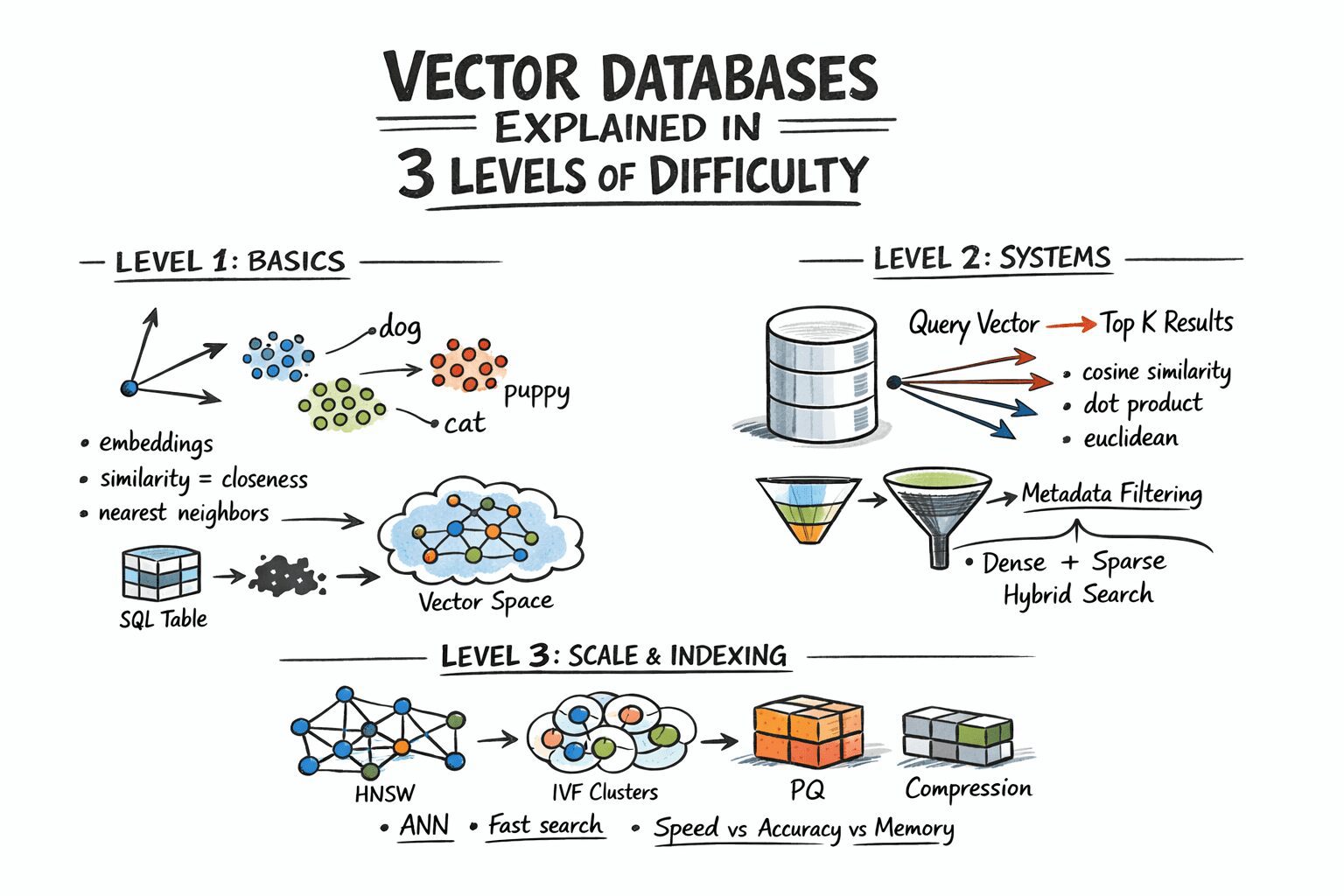
Structured data fits neatly into rows and columns. Unstructured data—text, images, audio—doesn’t. Embedding models like OpenAI’s text-embedding-3-small solve this by turning content into vectors. For example, the words “dog” and “puppy” become vectors that sit close in a 1536-dimensional space. A photo of a cat and a drawing of a cat also cluster together. This geometric similarity enables searches like “find me the 10 vectors closest to this query.”
Why Exact Search Fails
Brute-force comparison of a query vector against every stored vector works for small datasets. At scale, it’s impractical. A million vectors with 1536 dimensions each require billions of operations per query. This is where approximate nearest neighbor (ANN) algorithms step in, trading a tiny bit of accuracy for massive speed gains.
Level 2: Storing and Querying Vectors
Embeddings and Distance Metrics
Embedding models generate dense vectors (256–4096 dimensions). The specific numbers matter less than their geometry. Three common distance metrics include:
- Cosine similarity: Measures angles between vectors, ideal for text.
- Euclidean distance: Measures straight-line distance, useful when magnitude matters.
- Dot product: Fast and effective for normalized vectors.
Hybrid Search: Dense + Sparse
Pure vector search can miss keyword-level precision. A query for “GPT-5 release date” might drift toward general AI topics. Hybrid search combines dense vectors (ANN) with sparse methods (BM25) using reciprocal rank fusion (RRF). This blend captures both semantic understanding and keyword accuracy.
Metadata Filtering
Real-world queries often include filters: “Find similar documents created by this user after 2023.” Pre-filtering applies metadata rules first, then runs ANN on the subset. Post-filtering does the reverse. Pre-filtering is more accurate but slower. Most systems use smart indexing to balance speed and precision.
Level 3: Scaling with Indexing Algorithms
Hierarchical Navigable Small World (HNSW)
HNSW builds a multi-layer graph where vectors are nodes. Higher layers enable fast traversal; lower layers refine results. It’s fast and memory-heavy, making it ideal for high-accuracy applications. Parameters like ef_construction and M control tradeoffs between speed, memory, and recall.
Inverted File Index (IVF)
IVF clusters vectors using k-means, then searches only the nearest clusters. It uses less memory than HNSW but requires a training step. Pairing it with product quantization (IVF-PQ) compresses vectors 4–32x, enabling billion-scale datasets.
Product Quantization (PQ)
PQ compresses vectors by dividing them into subvectors and quantizing each to a codebook. This reduces memory usage significantly. Systems like Faiss combine IVF and PQ for efficient large-scale search.
Conclusion
Vector databases solve the problem of searching unstructured data by turning it into vectors and using ANN algorithms. From basic similarity search to hybrid retrieval and indexing strategies, they enable real-time queries at scale. Whether you’re building a recommendation engine or a document search tool, understanding these layers helps you choose the right tools for your use case. Ready to dive deeper? Share your thoughts in the comments!